Interactive Image Processing Graphs
Here you can explore a few Desmos graphs featuring gamma correction (using power law) and Linear Contrast Stretching.
Interactive Image Processing Graphs
Here you can explore a few Desmos graphs featuring gamma correction (using power law) and Linear Contrast Stretching.
Interactive Image Processing Graphs
Here you can explore a few Desmos graphs featuring gamma correction (using power law) and Linear Contrast Stretching.
Here you can explore several Desmos graphs featuring distributions, permutations/combinations, and regression. For the best experience, view these graphs on a computer rather than a phone.
Here you can explore several Desmos graphs featuring distributions, permutations/combinations, and regression. For the best experience, view these graphs on a computer rather than a phone.
Here you can explore several Desmos graphs featuring distributions, permutations/combinations, and regression. For the best experience, view these graphs on a computer rather than a phone.
Java Linear Algebra Uses
Contents
Getting Started
First, ensure you have the Jar file downloaded and added to your Java project. You can download the file here. You can also review the documentation for the library here. Once you have done that, create a class and begin using the library.
Creating a Complex Number
This library can handle real or complex matrices. So if you would like to create a complex matrix, you will need to know how to create a complex number. Begin by importing linalg.complex_number.CNumber.
Now we can begin creating complex numbers. Several constructors are offered to facilitate the creation of complex numbers. Here are some basic ones.

And here we can see each of the numbers created by printing them out.
You can also create complex numbers with Strings. Here are some examples.
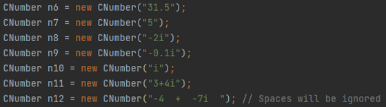
Here we can see each of the numbers created using the String constructors.
Creating a Matrix
The first thing you will need to do is import the linalg package at the top of your file so you can use the classes in the package. Most methods in the library are accessed through the Matrix class.
There are many constructors offered. We will begin by showcasing some of the basic ones.

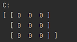
Here are the matrices created from each of these constructors.
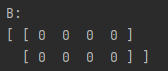
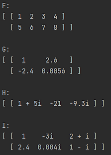
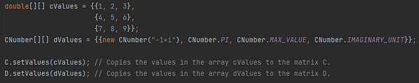
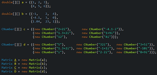
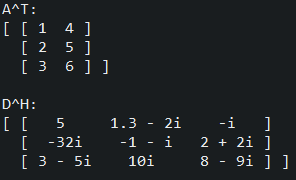
It is also possible to create matrices from data, specifically 2D arrays. These arrays can be of type int, double, String (following the style of the complex number String constructors), or CNumber. If you are going to use a CNumber array, ensure that you have imported linalg.complex_number.CNumber. Below are some examples of creating a matrices with 2D arrays.
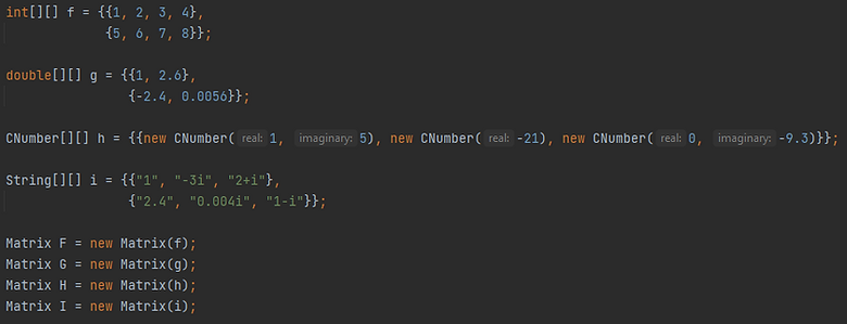
And here are the resulting matrices.
Manipulating Matrices
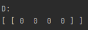
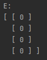
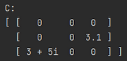
After a matrix has been constructed, you can manipulate the values in several ways. We will work with the four zero matrices B, C, D, and E that were created in the previous section. Each example will be working with the respective zero matrix. First, you can set the value at a specified index of a matrix.
Now we can print out the matrices and see the results.
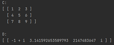
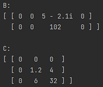
Rather than setting one element at a time, it is possible to set the values of the entire array at once, using an array. Note that the array must have the same dimensions as the matrix.
Here are the updated matrices.
You can also set a section or "slice" of a matrix by specifying the starting index for the row and column and for the upper left of the matrix containing the new values. The matrix of new values must fit in the matrix based on the starting indices.
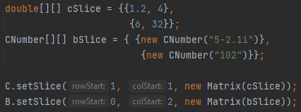
And here are the updated matrices.
You can also use the setCol() and setRow() methods similarly by passing a 1D array or a Vector. For more see the documentation.
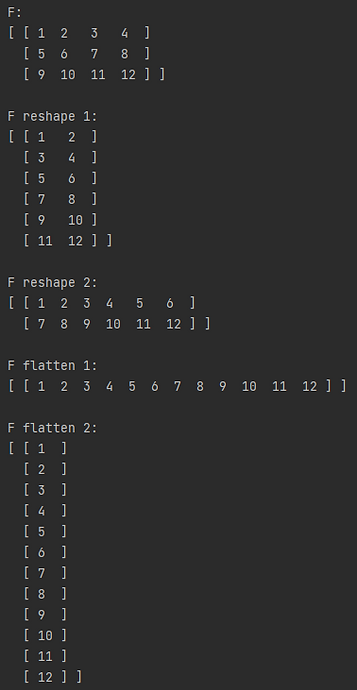
You can also reshape and flatten a matrix. The reshape method will change the dimensions of the matrix. Note, the new dimensions must have the same number of elements as the original matrix. The flatten method will flatten the matrix to have either a single row or a single column vector.
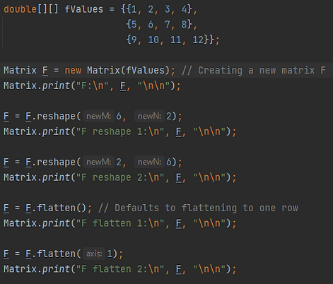
Here is the output of the above program.
There are many other manipulations that can be performed on matrices including, converting to a diagonal matrix, a triangular matrix, an upper Hessenburg matrix, swapping rows and columns, and removing rows and columns. For more on these functions see the documentation.
Operations With Matrices
First, we will create some matrices to use for the following matrix operations examples.
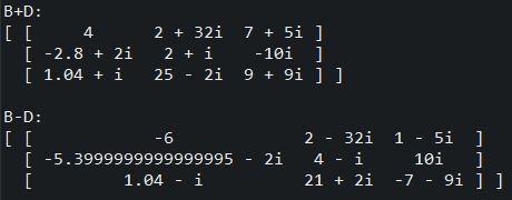
Next, we will see examples of the simple arithmetic operations addition and subtraction. For these two operations, the matrices must have the same shape.
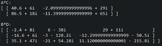
We can also multiply two matrices if the number of columns in the first matrix matches the number of rows in the second matrix.
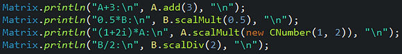
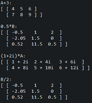
These operations, along with division, can also be performed with scalar values.
There is also the ability to transpose or conjugate-transpose (Hermation adjoint) a matrix. Note, if the transpose is applied to a complex matrix it will not take the complex conjugate.
It is possible to easily compute the Frobenius inner product between two matrices.
Also, determinants can be computed for real or complex matrices.
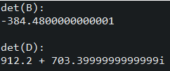
These are just a few examples of operations that can be performed using this library. For more operations see the documentation.
Solving Systems of Equations
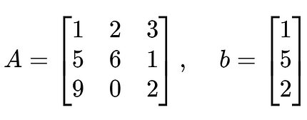
Solving a system of equations is a breeze using this library. The hardest part is forming the coefficient matrix and vector of constants. Consider the following system of equations and the corresponding coefficient matrix and vector of constants.

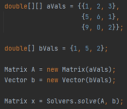
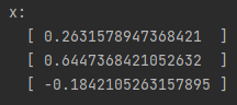
We can then create the matrix A and the vector b using the library. Then, we can use the Solver class to solve the system. The results are stored in a Matrix (or Vector if desired) x and printed out.
You can also solve a system using various decompositions and the forward and backward solve methods if you desired. See documentation for these methods.
Matrix Decompositions
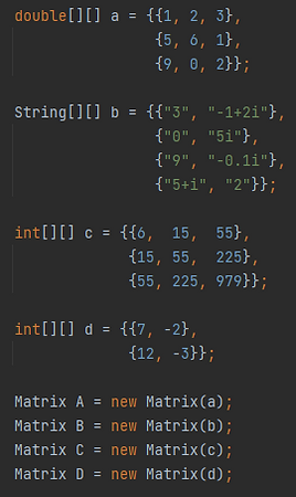
This library provides several matrix decompositions. Some of the important ones are listed here. See below for the matrices that will be used throughout the Matrix Decomposition section.
LU Decomposition
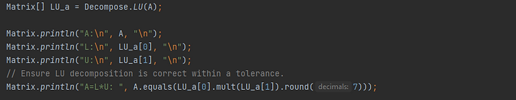
The LU Decomposition decomposes a matrix A into a unit lower diagonal matrix and an upper diagonal matrix. That is A=LU. The code below decomposes the matrix A into L and U. Then A, L, and U are printed out. Then, to ensure that the decomposition is correct, we check if L times U is equal to A. Because floating-point arithmetic can introduce small errors, we round the result of L times U.
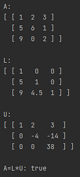
The results of this program are shown below.
The PA=LU and PAQ=LU decompositions are also available in this library. See the documentation for more.
QR Decomposition
The QR Decomposition decomposes a matrix A into an orthogonal (or possibly unitary if complex) matrix Q and an upper triangular matrix R. That is A=QR. The code below computes the QR decomposition of the matrix A and prints out A, Q, and R. Then, to ensure that the decomposition is correct, we check that A=QR (within 7 decimal places to account for floating-point error) and that Q is orthogonal.
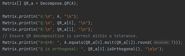
Here are the results of the program.

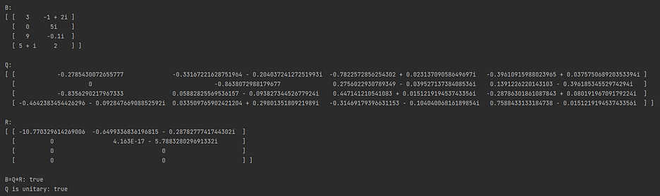
We can also compute the QR decomposition of a non-square and/or complex matrix. We will compute the QR decomposition of matrix B as an example using the code below. To ensure the decomposition is correct, we check that B=QR (within 7 decimal places to account for floating-point error) and that Q is unitary.
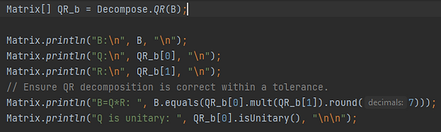
And here is the output of the program.
Cholesky Decomposition
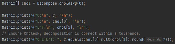
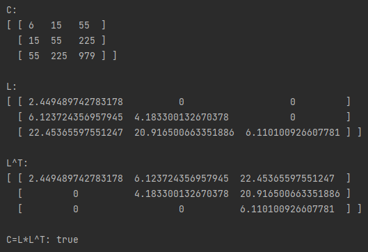
The Cholesky decomposition decomposes a Hermitian, positive-definite matrix C into the product of a lower triangular matrix L and its conjugate transpose L*. That is C=LL*. See the code below for an example of computing the Cholesky decomposition of the matrix C.
Schur Decomposition
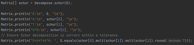
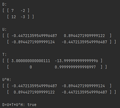
The Schur decomposition decomposes a matrix D into the product of a unitary matrix U (such that the columns of U are the eigenvectors of D), an upper triangular matrix T (with the eigenvalues of D along the diagonal) in complex/real Schur form and the conjugate transpose of U. That is D=UTU* By default, T will be in the complex Schur form. An additional boolean argument can be passed to Decompose.schur(Matrix, boolean). If set to false, T will be in real Schur form. The code below provides an example of computing the Schur decomposition of the matrix D. We verify the product UTU* equals D (within 7 decimal places to account for floating-point error).
And here is the output of the program.
Eigenvalues and Eigenvectors
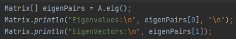
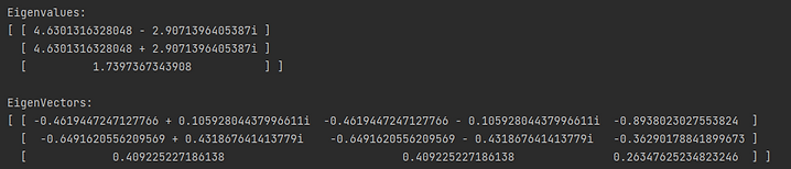
Computing eigenvalues and eigenvectors is trivial using this library. You could compute the Schur decomposition and extract the eigenvalues and vectors but there are also dedicated methods for finding the eigenvalues and eigenvectors. The example below demonstrates finding the eigenvalues and eigenvectors separately.


Both the eigenvalues and eigenvectors can be computed at the same time. See code below for an example.